Chi-Squared Tests (aka Goodness of Fit)

Chi-Squared Tests for Goodness of Fit

This 58 slide PowerPoint presentation covers the content of “Chi-squared Tests” within Edexcel Further Statistics 1 (Chapter 6 of the official Pearson FS1 textbook).
Each slide is accompanied by teacher notes.

[A free preview PowerPoint slideshow, containing approximately half the slides, is also available.]

We start with a general introduction for how you quantity the closeness of observed frequencies to the frequencies expected for a chosen standard distribution i.e. how to calculate Pearson’s Cumulative Test Statistic, X^2.

Both methods of calculating X^2 are covered.

In order to properly understand the concept of “Degrees of Freedom”, additional examples are included to fully explain how we determine the degrees of freedom of a given dataset by taking into account restrictions placed upon it. In my opinion, this is handled poorly by the textbook.

The loss of degrees of freedom due to having to combine adjacent columns of the dataset (because the observed/expected frequencies are too low), and because the observed data itself is needed to calculated a required parameter of the model distribution is also covered.

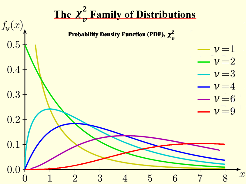
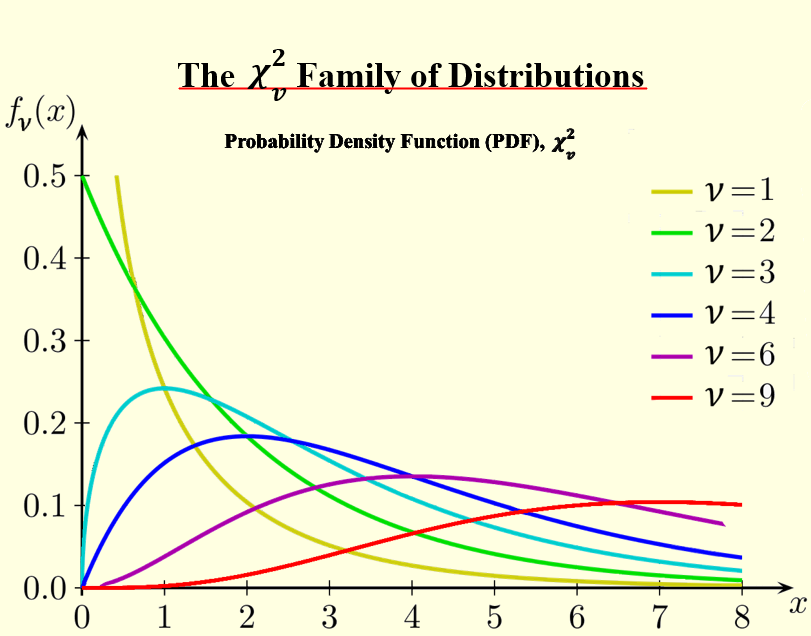
We then link this to our existing knowledge of Hypothesis Tests, and introduce the Chi-squared family of distribution. This section has also been extended to ensure that students properly understand how the chi-squared graphs vary with the data’s degrees of freedom, ν, and how to effectively these graphs (either by using the table “Percentage Points of the Chi-Squared Distribution” in the formula book or by using a calculator e.g. the Casio CG50).

Once we have the foundations in place, we use them to work through exam-style examples, comparing the given observed data to a chosen standard model distribution. For each example, we perform a hypothesis test to determine if there is sufficient evidence, at the required significance level, to reject null hypothesis.

The examples cover the following standard distributions:

• Discrete Uniform Distribution
• Geometric Distribution
• Binomial Distribution
• Poisson Distribution
  _

All examples are either newly created or significantly modified from past paper questions.

For each standard distribution we explain how to determine the probability of each outcome and, hence, the expected frequencies. We also explain how to, if necessary, estimate a required parameter (e.g. ρ for the Binomial distribution, λ for the Poisson Distribution) from the observed data.

The presentation, unlike the textbook, deals with the four standard, discrete distributions in turn i.e. it does not delay the section on the Geometric Distribution until the end. Instead, the section on continency tables is left to the end and given its proper title of “The Chi-Squared Test of Independence”.
In addition, the presentation contains detailed examples showing how to use the Casio CG50 calculator to perform Chi-Squared tests.

Regards

Gerard